Including inter-species measurements in differential expression analysis of RNAseq data with the compcodeR package

Paul Bastide & Mélina Gallopin

2024-07-14

library(compcodeR)
#> Loading required package: sm
#> Package 'sm', version 2.2-6.0: type help(sm) for summary information

Introduction

The compcodeR R package can generate RNAseq counts data and compare the relative performances of various popular differential analysis detection tools (Soneson and Delorenzi (2013)).

Using the same framework, this document shows how to generate “orthologous gene” (OG) expression for different species, taking into account their varying lengths, and their phylogenetic relationships, as encoded by an evolutionary tree.

This vignette provides a tutorial on how to use the “phylogenetic” functionalities of compcodeR. It assumes that the reader is already familiar with the compcodeR package vignette.

The phyloCompData class

The phyloCompData class extends the compData class of the compcodeR package to account for phylogeny and length information needed in the representation of OG expression data.

A phyloCompData object contains all the slots of a compData object, with an added slot containing a phylogenetic tree with ape format phylo, and a length matrix. It can also contain some added variable information, such as species names. More detailed information about the phyloCompData class are available in the section on the phylo data object. After conducting a differential expression analysis, the phyloCompData object has the same added information than the compData object (see the result object in the compcodeR package vignette).

A sample workflow

The workflow for working with the inter-species extension is very similar to the already existing workflow of the compcodeR package. In this section, we recall this workflow, stressing out the added functionalities.

Phylogenetic Tree

The simulations are performed following the description by Bastide et al. (2022).

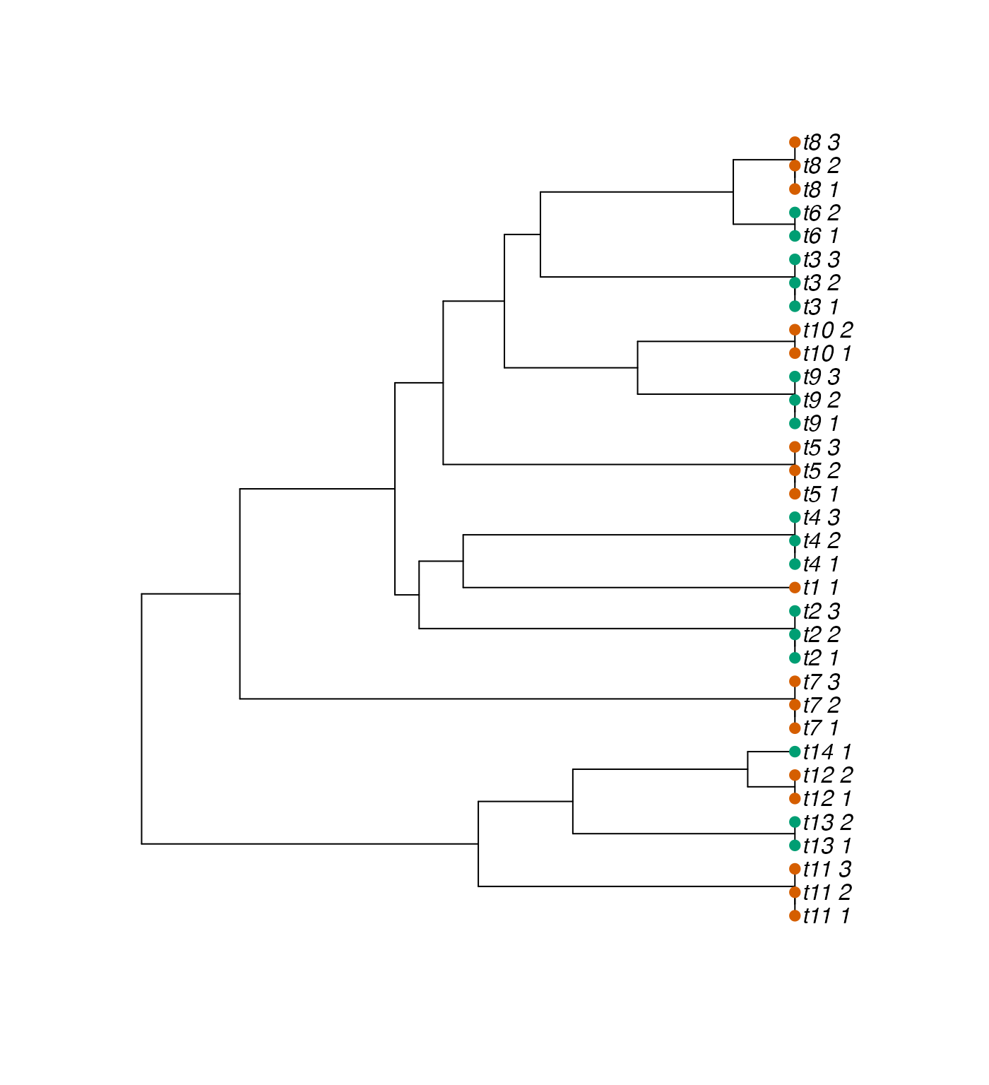
We use here the phylogenetic tree issued from Stern et al. (2017), normalized to unit height, that has $14$ species with up to 3 replicates, for a total number of sample equal to $34$ (see Figure below).

library(ape)
tree <- system.file("extdata", "Stern2018.tree", package = "compcodeR")
tree <- read.tree(tree)

Note that any other tree could be used, for instance randomly generated using a birth-death process, see e.g. function rphylo in the ape package.

Condition Design

To conduct a differential analysis, each species must be attributed a condition. Because of the phylogenetic structure, the condition design does matter, and have a strong influence on the data produced. Here, we assume that the conditions are mapped on the tree in a balanced way (“alt” design), which is the “best case scenario”.

# link each sample to a species
id_species <- factor(sub("_.*", "", tree$tip.label))
names(id_species) <- tree$tip.label
# Assign a condition to each species
species_names <- unique(id_species)
species_names[c(length(species_names)-1, length(species_names))] <- species_names[c(length(species_names), length(species_names)-1)]
cond_species <- rep(c(1, 2), length(species_names) / 2)
names(cond_species) <- species_names
# map them on the tree
id_cond <- id_species
id_cond <- cond_species[as.vector(id_cond)]
id_cond <- as.factor(id_cond)
names(id_cond) <- tree$tip.label

We can plot the assigned conditions on the tree to visualize them.

plot(tree, label.offset = 0.01)
tiplabels(pch = 19, col = c("#D55E00", "#009E73")[id_cond])

Phylogenetic tree with $14$ species and $34$ samples, with two conditions

Simulating data

Using this tree with associated condition design, we can then generate a dataset using a “phylogenetic Poisson Log Normal” (pPLN) distribution. We use here a Brownian Motion (BM) model of evolution for the latent phylogenetic log normal continuous trait, and assume that the phylogenetic model accounts for $90\%$ of the latent trait variance (i.e. there is an added uniform intra-species variance representing $10\%$ of the total latent trait variation). Using the "auto" setup, the counts are simulated so that they match empirical moments found in Stern and Crandall (2018). OG lengths are also drawn from a pPLN model, so that their moments match those of the empirical dataset of Stern and Crandall (2018). We choose to simulate $2000$ OGs, $10\%$ of which are differentially expressed, with an effect size of $3$.

The following code creates a phyloCompData object containing the simulated data set and saves it to a file named "alt_BM_repl1.rds".

set.seed(12890926)
alt_BM <- generateSyntheticData(dataset = "alt_BM",
                                n.vars = 2000, samples.per.cond = 17,
                                n.diffexp = 200, repl.id = 1,
                                seqdepth = 1e7, effect.size = 3,
                                fraction.upregulated = 0.5,
                                output.file = "alt_BM_repl1.rds",
                                ## Phylogenetic parameters
                                tree = tree,                      ## Phylogenetic tree
                                id.species = id_species,          ## Species structure of samples
                                id.condition = id_cond,           ## Condition design
                                model.process = "BM",             ## The latent trait follows a BM
                                prop.var.tree = 0.9,              ## Tree accounts for 90% of the variance
                                lengths.relmeans = "auto",        ## OG length mean and dispersion
                                lengths.dispersions = "auto")     ## are taken from an empirical exemple

The summarizeSyntheticDataSet works the same way as in the base compcodeR package, generating a report that summarize all the parameters used in the simulation, and showing some diagnostic plots.

summarizeSyntheticDataSet(data.set = "alt_BM_repl1.rds", 
                          output.filename = "alt_BM_repl1_datacheck.html")

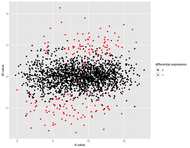
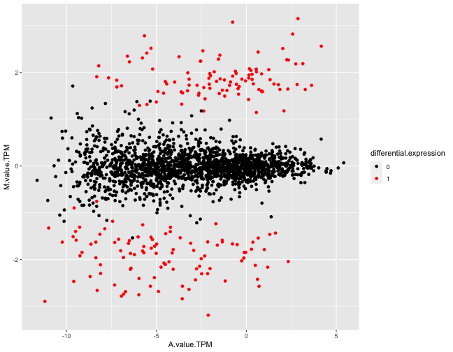
When applied to a phyloCompData object, it provides some extra diagnostics, related to the phylogenetic nature of the data. In particular, it contains MA-plots with TPM-normalized expression levels to take OG length into account, which generally makes the original signal clearer.

Example figures from the summarization report generated for a simulated data set. The top panel shows an MA plot, with the genes colored by the true differential expression status. The bottom panel shows the same plot, but using TPM-normalized estimated expression levels.

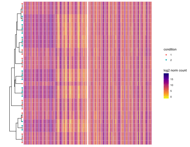
It also shows a log2 normalized counts heatmap plotted along the phylogeny, illustrating the phylogenetic structure of the differentially expressed OGs.

Example figures from the summarization report generated for a simulated data set. The tips colored by true differential expression status. Only the first 400 genes are represented. The first block of 200 genes are differencially expressed between condition 1 and 2. The second block of 200 genes are not differencially expressed.

Performing differential expression analysis

Differential expression analysis can be conducted using the same framework used in the compcodeR package, through the runDiffExp function.

All the standard methods can be used. To account for the phylogenetic nature of the data and for the varying length of the OGs, some methods have been added to the pool.

The code below applies three differential expression methods to the data set generated above: the DESeq2 method adapted for varying lengths, the log2(TPM) transformation for length normalization, combined with limma, using the trend empirical Bayes correction, and accounting for species-related correlations, and the phylogenetic regression tool phylolm applied on the same log2(TPM).

runDiffExp(data.file = "alt_BM_repl1.rds",
           result.extent = "DESeq2", Rmdfunction = "DESeq2.createRmd",
           output.directory = ".",
           fit.type = "parametric", test = "Wald")
runDiffExp(data.file = "alt_BM_repl1.rds",
           result.extent = "lengthNorm.limma", Rmdfunction = "lengthNorm.limma.createRmd",
           output.directory = ".",
           norm.method = "TMM",
           length.normalization = "TPM",
           data.transformation = "log2",
           trend = FALSE, block.factor = "id.species")
runDiffExp(data.file = "alt_BM_repl1.rds",
           result.extent = "phylolm", Rmdfunction = "phylolm.createRmd",
           output.directory = ".",
           norm.method = "TMM",
           model = "BM", measurement_error = TRUE,
           extra.design.covariates = NULL,
           length.normalization = "TPM",
           data.transformation = "log2")

As for a regular compcodeR analysis, example calls are provided in the reference manual (see the help pages for the runDiffExp function), and a list of all available methods can be obtained with the listcreateRmd() function.

listcreateRmd()
#>  [1] "DESeq2.createRmd"              
#>  [2] "DESeq2.length.createRmd"       
#>  [3] "DSS.createRmd"                 
#>  [4] "EBSeq.createRmd"               
#>  [5] "edgeR.exact.createRmd"         
#>  [6] "edgeR.GLM.createRmd"           
#>  [7] "lengthNorm.limma.createRmd"    
#>  [8] "lengthNorm.sva.limma.createRmd"
#>  [9] "logcpm.limma.createRmd"        
#> [10] "NBPSeq.createRmd"              
#> [11] "NOISeq.prenorm.createRmd"      
#> [12] "phylolm.createRmd"             
#> [13] "sqrtcpm.limma.createRmd"       
#> [14] "TCC.createRmd"                 
#> [15] "ttest.createRmd"               
#> [16] "voom.limma.createRmd"          
#> [17] "voom.ttest.createRmd"

Comparing results from several differential expression methods

Given that the phyloCompData object has the same structure with respect to the slots added by the differential expression analysis (see the result object, the procedure to compare results from several differential expression methods is exactly the same as for a compData object, and can be found in the corresponding section section of the compcodeR vignette.

Using your own data

As for a compData object, it is still possible to input user-defined data to produce a phyloCompData object for differential expression methods comparisons. One only needs to provide the additional information needed, that is the phylogenetic tree, and the length matrix. The constructor method will make sure that the tree is consistent with the count and length matrices, with the same dimensions and consistent species names.

## Phylogentic tree with replicates
tree <- read.tree(text = "(((A1:0,A2:0,A3:0):1,B1:1):1,((C1:0,C2:0):1.5,(D1:0,D2:0):1.5):0.5);")
## Sample annotations
sample.annotations <- data.frame(
  condition = c(1, 1, 1, 1, 2, 2, 2, 2),                 # Condition of each sample
  id.species = c("A", "A", "A", "B", "C", "C", "D", "D") # Species of each sample
  )
## Count Matrix
count.matrix <- round(matrix(1000*runif(8000), 1000))
## Length Matrix
length.matrix <- round(matrix(1000*runif(8000), 1000))
## Names must match
colnames(count.matrix) <- colnames(length.matrix) <- rownames(sample.annotations) <- tree$tip.label
## Extra infos
info.parameters <- list(dataset = "mydata", uID = "123456")
## Creation of the object
cpd <- phyloCompData(count.matrix = count.matrix,
                     sample.annotations = sample.annotations,
                     info.parameters = info.parameters,
                     tree = tree,
                     length.matrix = length.matrix)
## Check
check_phyloCompData(cpd)
#> [1] TRUE

Providing your own differential expression code

To use your own differential expression code, you can follow the base compcodeR instructions in the compcodeR vignette.

The extended data object

The phylocompData data object is an S4 object that extends the compData object, with the following added slots:

• tree [class phylo] (mandatory) – the phylogenetic tree describing the relationships between samples.

• length.matrix [class matrix] (mandatory) – the OG length matrix, with rows representing genes and columns representing samples.

• When produced with generateSyntheticData, the sample.annotations data frame has added column:

  • id.species [class character or numeric] – the species for each sample. Should match with the tip.label of the tree slot.

• When produced with generateSyntheticData, the variable.annotations data frame has an added columns:

  • lengths.relmeans [class numeric] – the true mean values used in the simulations of the OG lengths.
  • lengths.dispersions [class numeric] – the true dispersion values used in the simulations of the OG lengths.
  • M.value.TPM [class numeric] – the estimated log2-fold change between conditions 1 and 2 for each OG using TPM length normalization.
  • A.value.TPM [class numeric] – the estimated average expression in conditions 1 and 2 for each OG using TPM length normalization.
  • prop.var.tree [class numeric] – the proportion of the variance explained by the phylogeny for each gene.

The same way as the compData object, the phyloCompData object needs to be saved to a file with extension .rds.

The evaluation metrics

The evaluation metrics are unchanged, and described in the corresponding section section of the compcodeR vignette.

Session info

sessionInfo()
#> R version 4.4.1 (2024-06-14)
#> Platform: aarch64-apple-darwin20
#> Running under: macOS Sonoma 14.5
#> 
#> Matrix products: default
#> BLAS:   /Library/Frameworks/R.framework/Versions/4.4-arm64/Resources/lib/libRblas.0.dylib 
#> LAPACK: /Library/Frameworks/R.framework/Versions/4.4-arm64/Resources/lib/libRlapack.dylib;  LAPACK version 3.12.0
#> 
#> locale:
#> [1] en_US.UTF-8/en_US.UTF-8/en_US.UTF-8/C/en_US.UTF-8/en_US.UTF-8
#> 
#> time zone: UTC
#> tzcode source: internal
#> 
#> attached base packages:
#> [1] stats     graphics  grDevices utils     datasets 
#> [6] methods   base     
#> 
#> other attached packages:
#> [1] ape_5.8          compcodeR_1.41.0 sm_2.2-6.0      
#> [4] BiocStyle_2.33.1
#> 
#> loaded via a namespace (and not attached):
#>  [1] tidyselect_1.2.1     timeDate_4032.109   
#>  [3] dplyr_1.1.4          bitops_1.0-7        
#>  [5] fastmap_1.2.0        promises_1.3.0      
#>  [7] digest_0.6.36        rpart_4.1.23        
#>  [9] mime_0.12            lifecycle_1.0.4     
#> [11] cluster_2.1.6        statmod_1.5.0       
#> [13] ROCR_1.0-11          magrittr_2.0.3      
#> [15] compiler_4.4.1       rlang_1.1.4         
#> [17] sass_0.4.9           tools_4.4.1         
#> [19] utf8_1.2.4           yaml_2.3.9          
#> [21] knitr_1.48           statip_0.2.3        
#> [23] KernSmooth_2.23-24   timeSeries_4032.109 
#> [25] fBasics_4032.96      desc_1.4.3          
#> [27] grid_4.4.1           fansi_1.0.6         
#> [29] caTools_1.18.2       stabledist_0.7-1    
#> [31] xtable_1.8-4         colorspace_2.1-0    
#> [33] edgeR_4.3.4          ggplot2_3.5.1       
#> [35] scales_1.3.0         gtools_3.9.5        
#> [37] MASS_7.3-61          cli_3.6.3           
#> [39] rmarkdown_2.27       ragg_1.3.2          
#> [41] generics_0.1.3       cachem_1.1.0        
#> [43] stringr_1.5.1        parallel_4.4.1      
#> [45] stable_1.1.6         BiocManager_1.30.23 
#> [47] vctrs_0.6.5          jsonlite_1.8.8      
#> [49] bookdown_0.40        rmutil_1.1.10       
#> [51] clue_0.3-65          systemfonts_1.1.0   
#> [53] locfit_1.5-9.10      limma_3.61.2        
#> [55] jquerylib_0.1.4      spatial_7.3-17      
#> [57] glue_1.7.0           pkgdown_2.1.0.9000  
#> [59] stringi_1.8.4        gtable_0.3.5        
#> [61] later_1.3.2          shinydashboard_0.7.2
#> [63] munsell_0.5.1        tibble_3.2.1        
#> [65] pillar_1.9.0         htmltools_0.5.8.1   
#> [67] gplots_3.1.3.1       R6_2.5.1            
#> [69] textshaping_0.4.0    vioplot_0.5.0       
#> [71] evaluate_0.24.0      shiny_1.8.1.1       
#> [73] lattice_0.22-6       markdown_1.13       
#> [75] highr_0.11           png_0.1-8           
#> [77] modeest_2.4.0        httpuv_1.6.15       
#> [79] bslib_0.7.0          Rcpp_1.0.12         
#> [81] nlme_3.1-165         xfun_0.45           
#> [83] fs_1.6.4             zoo_1.8-12          
#> [85] pkgconfig_2.0.3

References

Bastide, Paul, Charlotte Soneson, Olivier Lespinet, and Mélina Gallopin. 2022. “Benchmark of Differential Gene Expression Analysis Methods for Inter-Species RNA-Seq Data Using a Phylogenetic Simulation Framework.” bioRxiv Preprint. https://doi.org/10.1101/2022.01.21.476612.

Soneson, Charlotte, and Mauro Delorenzi. 2013. “A Comparison of Methods for Differential Expression Analysis of RNA-seq Data.” BMC Bioinformatics 14: 91.

Stern, David B., Jesse Breinholt, Carlos Pedraza-Lara, Marilú López-Mejía, Christopher L. Owen, Heather Bracken-Grissom, James W. Fetzner, and Keith A. Crandall. 2017. “Phylogenetic Evidence from Freshwater Crayfishes That Cave Adaptation Is Not an Evolutionary Dead-End.” Evolution 71 (10): 2522–32. https://doi.org/10.1111/evo.13326.

Stern, David B., and Keith A. Crandall. 2018. “The Evolution of Gene Expression Underlying Vision Loss in Cave Animals.” Molecular Biology and Evolution 35 (8): 2005–14. https://doi.org/10.1093/molbev/msy106.