Introduction
The primary aim of the dreval package is to evaluate and
compare one or more reduced dimension representations, in terms of how
well they retain the structure from a reference representation. Here, we
illustrate its application to a single-cell RNA-seq data set of
peripheral blood mononuclear cells (PBMCs), representing a subset of the
pbmc3k data set from the TENxPBMCData package.
The set of genes has been subset to only highly variable ones, and
several dimension reduction methods (PCA, tSNE and UMAP) have been
applied.
data(pbmc3ksub)
pbmc3ksub
#> class: SingleCellExperiment
#> dim: 1804 2700
#> metadata(1): log.exprs.offset
#> assays(2): counts logcounts
#> rownames(1804): LYZ S100A9 ... AGTRAP ATXN1L
#> rowData names(3): ENSEMBL_ID Symbol_TENx Symbol
#> colnames(2700): Cell1 Cell2 ... Cell2699 Cell2700
#> colData names(11): Sample Barcode ... Individual Date_published
#> reducedDimNames(8): PCA PCA_k2 ... UMAP_nn15 UMAP_nn30
#> mainExpName: NULL
#> altExpNames(0):
Evaluation
The dreval() function is the main function in the
package, and calculates several metrics comparing each of the reduced
dimension representations in the SingleCellExperiment
object to the designed reference representation. Here, we use the
underlying normalized and log-transformed data contained in the
logcounts assay as the reference representation. For a list
of the calculated metrics, see the help page for
dreval().
Result visualization
The output of dreval() is a list with two elements. The
plots entry contains several diagnostic plot objects, while
the scores entry contains the calculated scores for each of
the evaluated reduced dimension representations. These can be summarized
visually with the plotRankSummary() function.
dre$scores
#>             Method dimensionality SpearmanCorrDist PearsonCorrDist KSStatDist
#> D...1          PCA             25        0.8154994       0.8573328  0.3444569
#> D...2       PCA_k2              2        0.6847185       0.6703615  0.5003768
#> D...3  TSNE_perp30              2        0.6529265       0.5634928  0.3798717
#> D...4   TSNE_perp5              2        0.4319733       0.3580134  0.3879359
#> D...5  TSNE_perp15              2        0.6082011       0.5531568  0.3824449
#> D...6 TSNE_perp100              2        0.6530342       0.5303586  0.4009860
#> D...7    UMAP_nn15              2        0.6295305       0.5729313  0.4337395
#> D...8    UMAP_nn30              2        0.6392410       0.5452490  0.4644088
#>       EuclDistBetweenDists SammonStress Trustworthiness_k10 Continuity_k10
#> D...1            0.2689303   0.07391334           0.9078543      0.8846762
#> D...2            0.5018734   0.26715742           0.8079315      0.8337003
#> D...3            0.3986876   0.16723525           0.8485094      0.8323802
#> D...4            0.4113424   0.17301868           0.8266943      0.7934712
#> D...5            0.3934171   0.16283086           0.8430795      0.8150423
#> D...6            0.4569962   0.22048310           0.8560838      0.8381717
#> D...7            0.5211990   0.29443922           0.8326147      0.8223748
#> D...8            0.5683829   0.34864929           0.8358089      0.8377692
#>       Trustworthiness_k75 Continuity_k75 MeanJaccard_k10 MeanJaccard_k75
#> D...1           0.9188758      0.9266787       0.1705789       0.4113410
#> D...2           0.8509984      0.8861510       0.1101979       0.3206625
#> D...3           0.8523844      0.8797668       0.1385658       0.3234358
#> D...4           0.7956347      0.8046975       0.1276278       0.2714622
#> D...5           0.8486944      0.8622888       0.1353894       0.3186285
#> D...6           0.8618369      0.8924744       0.1371832       0.3381405
#> D...7           0.8537153      0.8733586       0.1266815       0.3208645
#> D...8           0.8616588      0.8900690       0.1278621       0.3275634
#>       coRankingQlocal coRankingQglobal KmaxLCMC
#> D...1       0.3592266        0.2536750      115
#> D...2       0.2630986        0.1954727      122
#> D...3       0.2767429        0.1874120      120
#> D...4       0.2171358        0.1246179      106
#> D...5       0.2637424        0.1737807      114
#> D...6       0.2854750        0.1997314      116
#> D...7       0.2660368        0.1817096      116
#> D...8       0.2793017        0.1948339      120
suppressPackageStartupMessages({
  library(ggplot2)
})
cowplot::plot_grid(plotlist = lapply(dre$plots$disthex, function(w) w +
  theme(axis.title = element_text(size = 7))), ncol = 2)
#> Warning: `stat(density)` was deprecated in ggplot2 3.4.0.
#> ℹ Please use `after_stat(density)` instead.
#> ℹ The deprecated feature was likely used in the dreval package.
#>   Please report the issue at <https://github.com/csoneson/dreval/issues>.
#> This warning is displayed once per session.
#> Call `lifecycle::last_lifecycle_warnings()` to see where this warning was
#> generated.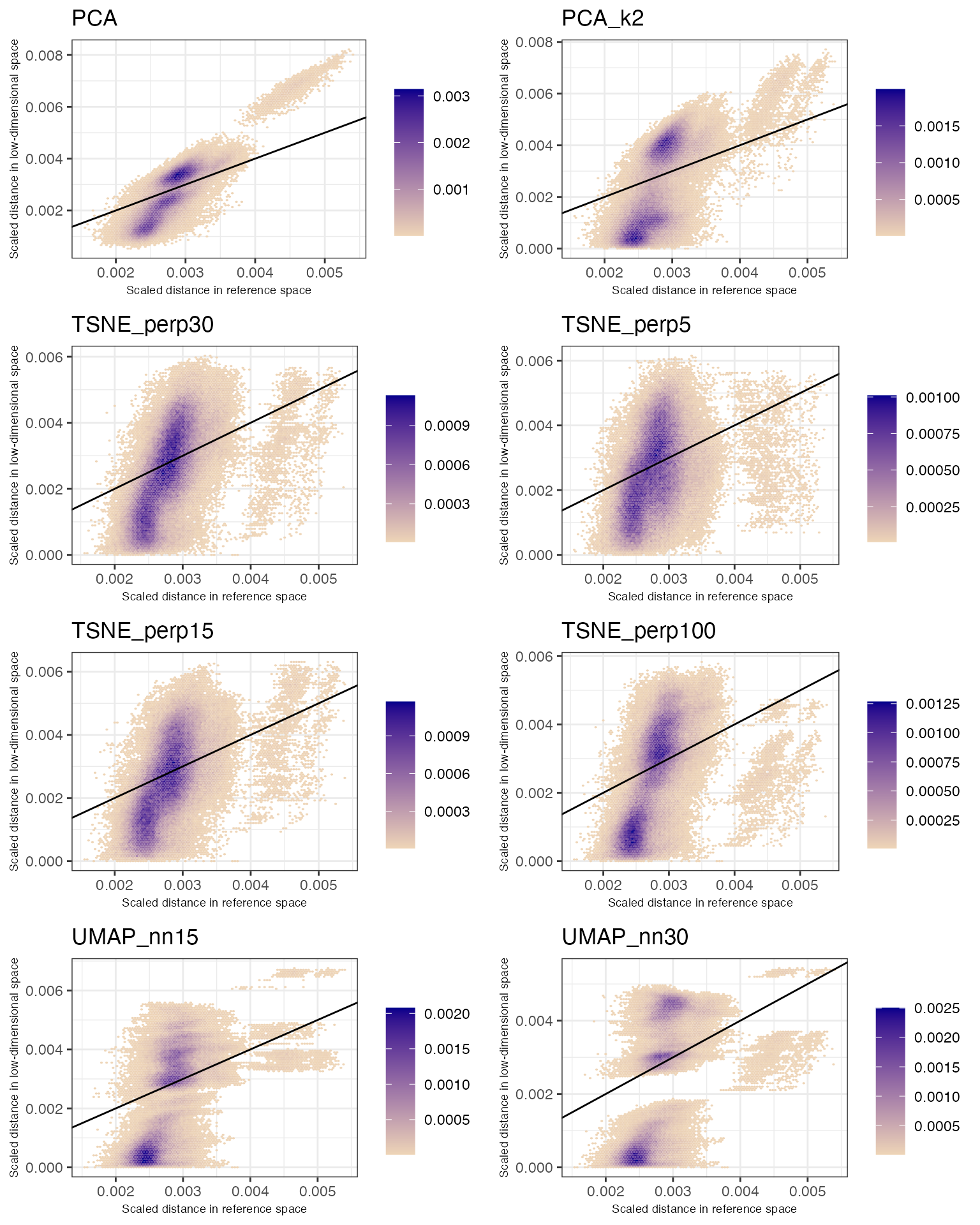
plotRankSummary(dre$scores) +
  theme(axis.text.x = element_text(angle = 45, hjust = 1, vjust = 1))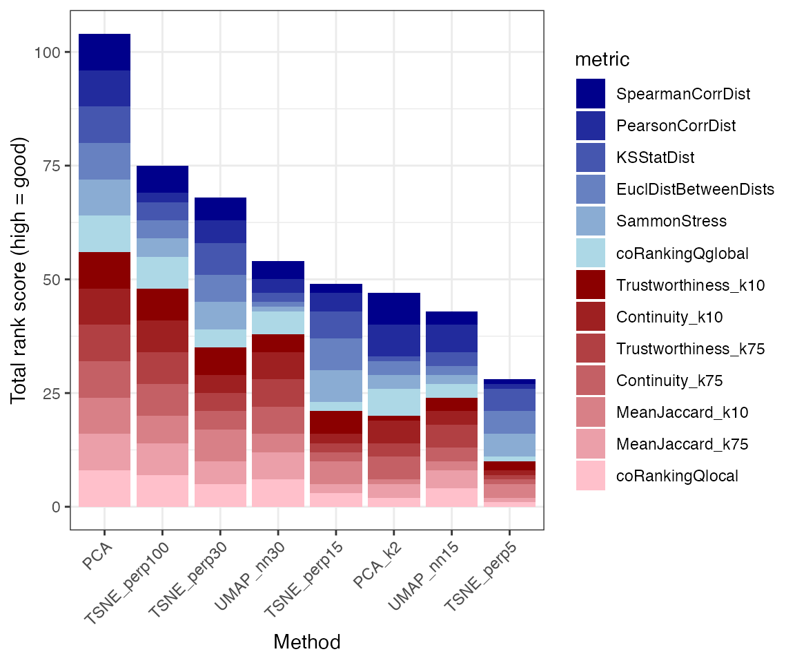
Using a reduced dimension representation as the reference space
In the example above, we used the original feature space (the
logcounts assay) as the reference space, to which all
reduced dimension representations were compared. It is also possible to
use one of the reduced dimension representations as the reference space,
as we will illustrate here.
dre <- dreval(
  sce = pbmc3ksub, refType = "dimred", refDimRed = "PCA",
  dimReds = NULL, nSamples = 500, kTM = c(10, 75),
  verbose = FALSE, distNorm = "l2"
)
dre$scores
#>             Method dimensionality SpearmanCorrDist PearsonCorrDist KSStatDist
#> D...1       PCA_k2              2        0.9233915       0.8942498  0.2644088
#> D...2  TSNE_perp30              2        0.7675047       0.7094667  0.1252665
#> D...3   TSNE_perp5              2        0.5943282       0.5488952  0.1078958
#> D...4  TSNE_perp15              2        0.7263592       0.6940593  0.1089699
#> D...5 TSNE_perp100              2        0.7851810       0.7114814  0.2111102
#> D...6    UMAP_nn15              2        0.7984050       0.7682800  0.3160000
#> D...7    UMAP_nn30              2        0.8475167       0.7620543  0.3751743
#>       EuclDistBetweenDists SammonStress Trustworthiness_k10 Continuity_k10
#> D...1            0.2897892    0.1138349           0.9010931      0.9417259
#> D...2            0.3186966    0.1071415           0.9591690      0.9607034
#> D...3            0.3812950    0.1500976           0.9401556      0.9386072
#> D...4            0.3224079    0.1130083           0.9538675      0.9540698
#> D...5            0.3555046    0.1353942           0.9630918      0.9671030
#> D...6            0.3808133    0.1843372           0.9508854      0.9564619
#> D...7            0.4192053    0.2220888           0.9535897      0.9631501
#>       Trustworthiness_k75 Continuity_k75 MeanJaccard_k10 MeanJaccard_k75
#> D...1           0.9403377      0.9574120       0.1821428       0.4777051
#> D...2           0.9379067      0.9463695       0.3427420       0.5432202
#> D...3           0.8737818      0.9015667       0.2960875       0.4513358
#> D...4           0.9259113      0.9379746       0.3246281       0.5226296
#> D...5           0.9495374      0.9564119       0.3597027       0.5686795
#> D...6           0.9429501      0.9511481       0.3181976       0.5445045
#> D...7           0.9443877      0.9551933       0.3204885       0.5482587
#>       coRankingQlocal coRankingQglobal KmaxLCMC
#> D...1       0.4315576        0.2709721      137
#> D...2       0.4883456        0.2697993       52
#> D...3       0.4176202        0.2046238       50
#> D...4       0.4683484        0.2539875       52
#> D...5       0.5039833        0.2913327       50
#> D...6       0.4683770        0.2737537       53
#> D...7       0.4691012        0.2962409       50
cowplot::plot_grid(plotlist = lapply(dre$plots$disthex, function(w) w +
  theme(axis.title = element_text(size = 7))), ncol = 2)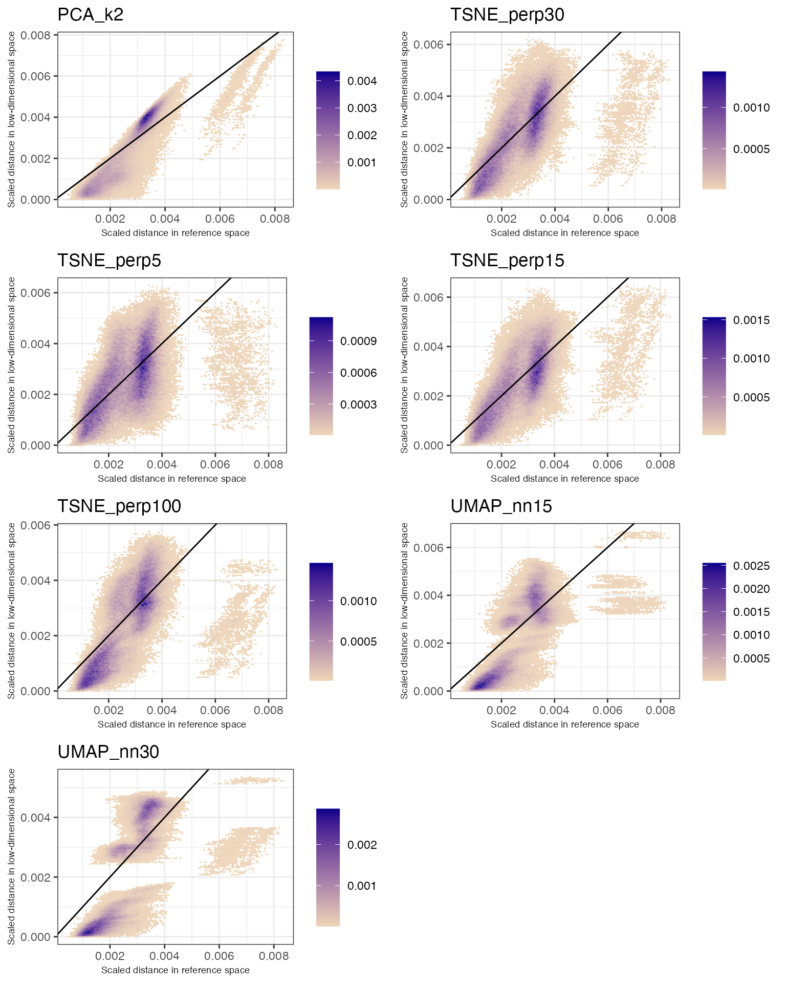
plotRankSummary(dre$scores) +
  theme(axis.text.x = element_text(angle = 45, hjust = 1, vjust = 1))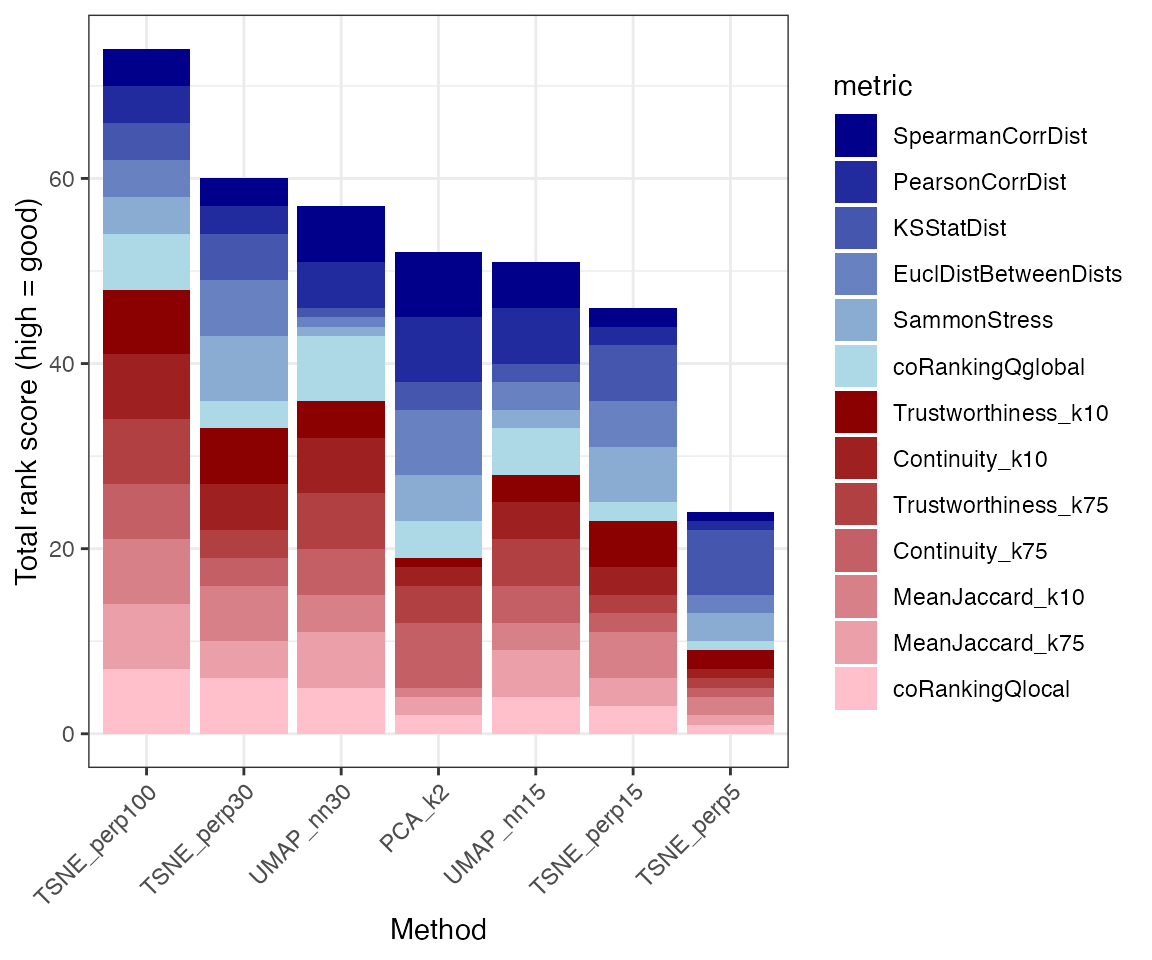
Computational efficiency
dreval relies heavily on the calculation of pairwise
distances among samples, and is consequently computationally demanding
for large data sets. The dreval() function allows for
subsampling a smaller number of samples, as well as selecting a subset
of the variables, to speed up calculations and reduce the memory
footprint. Here we illustrate that for the example data set, the
calculated metrics are stable under subsampling of cells.
suppressPackageStartupMessages({
  library(dplyr)
  library(tidyr)
  library(ggplot2)
})

set.seed(1)
nS <- c(100, 400, 1000, 1500, 2700)
v <- lapply(nS, function(n) {
  if (n == 2700) nR <- 1
  else nR <- 2
  lapply(seq_len(nR), function(i) {
    message(n, " samples, replicate ", i)
    dreval(sce = pbmc3ksub, refAssay = "logcounts", dimReds = NULL,
           nSamples = n, kTM = 50, verbose = FALSE)$scores %>%
      dplyr::mutate(nSamples = n, replicate = i)
  })
})
vv <- do.call(dplyr::bind_rows, v)

vv <- vv %>%
  tidyr::gather(
    key = "measure", value = "value",
    -Method, -dimensionality, -nSamples, -replicate
  )

suppressWarnings(
  ggplot(vv, aes(x = nSamples, y = value, color = Method)) +
    geom_point(size = 3) + facet_wrap(~ measure, scales = "free_y") +
    geom_smooth(se = FALSE) + theme_bw()
)
Session info
sessionInfo()
#> R version 4.6.0 (2026-04-24)
#> Platform: aarch64-apple-darwin23
#> Running under: macOS Sequoia 15.7.7
#>
#> Matrix products: default
#> BLAS:   /Library/Frameworks/R.framework/Versions/4.6/Resources/lib/libRblas.0.dylib
#> LAPACK: /Library/Frameworks/R.framework/Versions/4.6/Resources/lib/libRlapack.dylib;  LAPACK version 3.12.1
#>
#> locale:
#> [1] en_US.UTF-8/en_US.UTF-8/en_US.UTF-8/C/en_US.UTF-8/en_US.UTF-8
#>
#> time zone: UTC
#> tzcode source: internal
#>
#> attached base packages:
#> [1] stats     graphics  grDevices utils     datasets  methods   base
#>
#> other attached packages:
#> [1] ggplot2_4.0.3 dreval_0.1.6
#>
#> loaded via a namespace (and not attached):
#>  [1] SummarizedExperiment_1.42.0 gtable_0.3.6
#>  [3] xfun_0.59                   bslib_0.11.0
#>  [5] sparsesvd_0.2-3             Biobase_2.72.0
#>  [7] lattice_0.22-9              vctrs_0.7.3
#>  [9] tools_4.6.0                 generics_0.1.4
#> [11] stats4_4.6.0                tibble_3.3.1
#> [13] cluster_2.1.8.2             pkgconfig_2.0.3
#> [15] Matrix_1.7-5                RColorBrewer_1.1-3
#> [17] S7_0.2.2                    desc_1.4.3
#> [19] S4Vectors_0.50.1            lifecycle_1.0.5
#> [21] compiler_4.6.0              farver_2.1.2
#> [23] iotools_0.4-0               textshaping_1.0.5
#> [25] Seqinfo_1.2.0               coRanking_0.2.5
#> [27] htmltools_0.5.9             sass_0.4.10
#> [29] yaml_2.3.12                 hexbin_1.28.5
#> [31] pillar_1.11.1               pkgdown_2.2.0.9000
#> [33] jquerylib_0.1.4             tidyr_1.3.2
#> [35] MASS_7.3-65                 SingleCellExperiment_1.34.0
#> [37] DelayedArray_0.38.2         cachem_1.1.0
#> [39] abind_1.4-8                 tidyselect_1.2.1
#> [41] digest_0.6.39               dplyr_1.2.1
#> [43] purrr_1.2.2                 labeling_0.4.3
#> [45] cowplot_1.2.0               fastmap_1.2.0
#> [47] grid_4.6.0                  cli_3.6.6
#> [49] SparseArray_1.12.2          magrittr_2.0.5
#> [51] S4Arrays_1.12.0             withr_3.0.3
#> [53] scales_1.4.0                rmarkdown_2.31
#> [55] XVector_0.52.0              matrixStats_1.5.0
#> [57] otel_0.2.0                  ragg_1.5.2
#> [59] evaluate_1.0.5              knitr_1.51
#> [61] GenomicRanges_1.64.0        IRanges_2.46.0
#> [63] rlang_1.2.0                 Rcpp_1.1.1-1.1
#> [65] wordspace_0.2-9             glue_1.8.1
#> [67] BiocGenerics_0.58.1         jsonlite_2.0.0
#> [69] R6_2.6.1                    MatrixGenerics_1.24.0
#> [71] systemfonts_1.3.2           fs_2.1.0