Visualize design matrix

Given a sample table and a design formula, generate a collection of static plots for exploring the resulting design matrix graphically. This function is called internally by ExploreModelMatrix(), but can also be used directly if interactivity is not required.

VisualizeDesign(
  sampleData,
  designFormula = NULL,
  flipCoordFitted = FALSE,
  flipCoordCoocc = FALSE,
  textSizeFitted = 5,
  textSizeCoocc = 5,
  textSizeLabsFitted = 12,
  textSizeLabsCoocc = 12,
  lineWidthFitted = 25,
  addColorFitted = TRUE,
  colorPaletteFitted = scales::hue_pal(),
  dropCols = NULL,
  designMatrix = NULL
)

Arguments

sampleData

A data.frame of DataFrame with sample information.

designFormula

A formula. All components of the terms must be present as columns in sampleData.

flipCoordFitted, flipCoordCoocc

A logical, whether to flip the coordinate axes in the fitted values/co-occurrence plot, respectively.

textSizeFitted, textSizeCoocc

A numeric scalar giving the text size in the fitted values/co-occurrence plot, respectively.

textSizeLabsFitted, textSizeLabsCoocc

A numeric scalar giving the text size for the axis labels in the fitted values/co-occurrence plot, respectively.

lineWidthFitted

A numeric scalar giving the maximal length of a row in the fitted values plot, before it is split and printed on multiple lines

addColorFitted

A logical scalar indicating whether the terms in the fitted values plot should be shown in different colors.

colorPaletteFitted

A function returning a color palette to use for coloring the model coefficients in the fitted values plot.

dropCols

A character vector with columns to drop from the design matrix, or NULL if no columns should be dropped.

designMatrix

A numeric matrix, which can be supplied as an alternative to designFormula. Rows must be in the same order as the rows in sampleData.

Value

A list with the following elements:

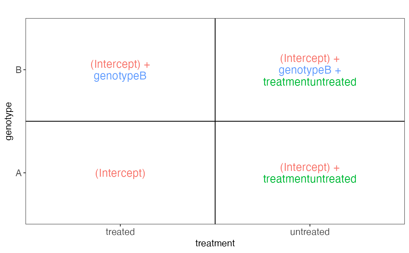
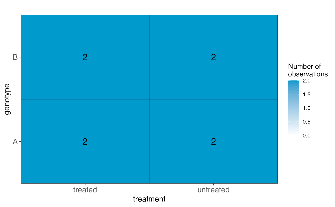
• sampledata: A data.frame, expanded from the input sampleData

• plotlist: A list of plots, displaying the fitted values for each combination of predictor values, in terms of the model coefficients.

• designmatrix: The design matrix, after removing any columns in dropCols

• pseudoinverse: The pseudoinverse of the design matrix

• vifs: A data.frame with calculated variance inflation factors

• colors: A vector with colors to use for different model coefficients

• cooccurrenceplots: A list of plots, displaying the co-occurrence pattern for the predictors (i.e., the number of observations for each combination of predictor values)

• totnbrrows: The total number of "rows" in the list of plots of fiitted values. Useful for deciding the required size of the plot canvas.

Details

Note that if a design matrix is supplied (via the designMatrix argument), caution is required in order to interpret especially the cooccurrence plot in the situation where the provided sampleData contains additional columns not used to generate the design matrix (or when it does not contain all the relevant columns).

Author

Charlotte Soneson

Examples

VisualizeDesign(
  sampleData = data.frame(genotype = rep(c("A", "B"), each = 4),
                          treatment = rep(c("treated", "untreated"), 4)),
  designFormula = ~genotype + treatment
)
#> $sampledata
#>   genotype treatment                                        value nSamples
#> 1        A   treated                                  (Intercept)        2
#> 2        A untreated             (Intercept) + treatmentuntreated        2
#> 3        B   treated                      (Intercept) + genotypeB        2
#> 4        B untreated (Intercept) + genotypeB + treatmentuntreated        2
#> 
#> $plotlist
#> $plotlist[[1]]

#> 
#> 
#> $designmatrix
#>   (Intercept) genotypeB treatmentuntreated
#> 1           1         0                  0
#> 2           1         0                  1
#> 3           1         0                  0
#> 4           1         0                  1
#> 5           1         1                  0
#> 6           1         1                  1
#> 7           1         1                  0
#> 8           1         1                  1
#> 
#> $pseudoinverse
#>                         1      2      3      4      5      6      7      8
#> (Intercept)         0.375  0.125  0.375  0.125  0.125 -0.125  0.125 -0.125
#> genotypeB          -0.250 -0.250 -0.250 -0.250  0.250  0.250  0.250  0.250
#> treatmentuntreated -0.250  0.250 -0.250  0.250 -0.250  0.250 -0.250  0.250
#> 
#> $vifs
#>          coefficient vif
#> 1          genotypeB   1
#> 2 treatmentuntreated   1
#> 
#> $colors
#>        (Intercept) treatmentuntreated          genotypeB 
#>          "#F8766D"          "#00BA38"          "#619CFF" 
#> 
#> $cooccurrenceplots
#> $cooccurrenceplots[[1]]

#> 
#> 
#> $totnbrrows
#> [1] 2
#>